Side-by-Side Animations in COMSOL: Visualize Multiple Plots in One Window

When you run a time-dependent coupled simulation, let's say, a Joule-heating problem where both temperature and electric potential evolve over time, exporting two separate animations and watching them separately is clunky. COMSOL gives you at least two clean ways to place multiple plot groups side by side inside a single animation. This article walks through both: the modern Array approach available since COMSOL 5.x, and the classic Deformation-node offset trick that still works perfectly in older models.

Setting the Scene

Assume you have a time-dependent study with at least two results of interest:

• A Surface plot of Current density (A/m^2) — typically living in a Current density (ec) plot group.

• A Surface plot of Electric Potential (V) — typically living in an Electric Potential (ec) plot group.

The goal is a single animation file that shows both fields simultaneously, with both fields updated frame by frame as time advances.

Method 1: The Plot Array Setting (Modern Way)

The Plot Array feature is built directly into every 2D (and 3D) Plot Group - no extra node to add. You enable it simply by left-clicking the plot group and expanding the Plot Array section at the bottom of its Settings panel.

Step 1 - Create a new 2D Plot Group

In the Results branch, right-click and choose 2D Plot Group (or 3D Plot Group if your geometry is 3D). Rename it something descriptive, for example, Side-by-Side I and V.

Step 2 - Enable Plot Array in the Settings panel

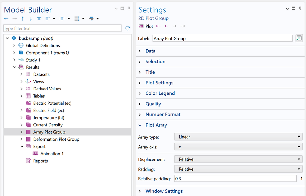
Left-click the new plot group to open its Settings panel on the right. Scroll down to the Plot Array section and configure it:

• Array type: Linear for a horizontal or vertical strip of panels.

• Array axis: x to place the panels side by side horizontally.

• Displacement: Relative (COMSOL spaces the panels automatically based on geometry size).

• Padding / Relative padding: controls the gap between panels; a value around 0.3 gives a comfortable spacing.

  
  

No separate node needs to be added - these settings live directly in the plot group.

Step 3 - Add your Surface plots to the plot group

Right-click the plot group and add a Surface plot. Set the expression to ec.normJ. In the Surface node's settings, find the Array Index field and set it to 1 - this pins the current density plot to the first panel.

Add a second Surface plot to the same plot group. Set the expression to V (or comp1.V) and set its Array Index to 2.

Give each surface plot a meaningful title through Title → Manual - something like Current density (A/m^2) and Electric Potential (V) - so the two panels are self-labeling in the exported animation.

Step 4 - Set the time parameter

In the plot group settings, ensure Parameter value (time) uses the solution time from your study. COMSOL usually fills this in automatically, but double-check that the dataset points to the correct Time-Dependent Solution.

Step 5 - Export as an animation

Right-click Export → Animation. Set:

• Output: MP4 or GIF, depending on your audience.

• Plot group: your new Side-by-Side I and V group.

• Frame selection: all times, or a range if you only need part of the simulation.

  
  

Click Export, and COMSOL will render every time step with both panels side by side.

Method 2: The Deformation Node Offset Trick (Classic Way)

Before the Array node existed — and still useful when you want finer manual control over exact placement — the standard workaround was to place both physics results into a single plot group and use a Deformation node on each surface to shift one of them sideways so they no longer overlap.

The Core Idea

A Deformation node normally displaces the rendered geometry by a vector field (used for structural mechanics visualizations). But you can exploit it with a constant displacement to simply translate a surface plot by a fixed offset in X or Y, effectively parking the two results next to each other.

Step 1 - Create a single 2D Plot Group

Right-click Results → 2D Plot Group. Rename it, for example, I and V Offset.

Step 2 - Add the first Surface (Current density)

Add a Surface node inside the plot group. Set the expression to T. Leave the deformation at its default (none). This plot will sit at the natural geometry position.

Step 3 - Add the second Surface (Voltage) with a Deformation

Add a second Surface node. Set the expression to V.

Right-click this second Surface node and choose Deformation. In the Deformation settings:

• Tick Specify deformation.

• Set the X-component to a constant equal to the width of your geometry plus a small gap. For example, if your model spans 0 to 0.1 m in X, enter 0.11 (in meters) to place the voltage plot just to the right of the temperature plot with a 1 mm gap.

• Leave the Y-component as 0.

  
  

The Deformation node will move the second surface to the right by that exact offset, placing it cleanly beside the first.

Step 4 - Adjust titles and color bars

Because both surfaces now share the same plot group, COMSOL will try to use a single shared color bar by default. To get independent color bars:

• Open each Surface node → Color Legend → enable Show legend.

• Under Range, untick Auto and set limits manually for each surface.

  
  

You may also want to add Annotations (right-click the plot group → Annotation) to label each panel with the field name and units, since the geometry position alone won't tell the viewer which panel is which.

Step 5 - Export the animation exactly as in Method 1

Right-click Export → Animation, select this plot group, choose your output format and frame range, and export.

Choosing Between the Two Methods

The Plot Array setting is almost always the better choice for new work. It keeps the two plots geometrically independent, handles color bars and titles cleanly, and does not require you to know or hard-code the physical size of your geometry. The Deformation offset approach is worth knowing because it works in any COMSOL version, and it gives you pixel-perfect control when you need a very specific layout. It can also be used for more than two fields: add a third Surface with a deformation of 2 × (width + gap) to create a row of three.

Both methods export into the same Animation node and support the same output formats, so the choice has no effect on downstream use of the animation files.

Running a time-dependent coupled simulation is hard enough on its own. At least the visualization side does not have to be: a few extra nodes in the Results tree and both fields animate together, frame by frame, in a single file.